Sequential Indicator Simulation of Lithofacies

This example demonstrates Multiple Indicator Simulation (MIS / SIS) using IndicatorKriging on a 2-D lithofacies dataset digitised from an outcrop photograph (Klingbeil 1998).

Four lithofacies are modelled as categorical indicator variables:

Code	Lithology	Proportion
C	Cobble	18 %
Cl	Clay	23 %
FS	Fine Sand	21 %
G	Gravel	38 %

SIS workflow

1. Convert raw category labels into K = 4 binary indicator datasets via set_categorical_obs().

2. Assign variograms to all K² = 16 pairs in one call using set_indicator_vgm(). Three cross strategies are available:

   • "same" — one shared sill for all K² pairs. Simplest; relies on post_solve normalisation to compensate for approximate cross-sills.

   • "proportional" — auto sills = p_k (1 − p_k); cross sills = √(s_k · s_l). LMC positive-definite for each nested structure; requires proportions.

   • "independent" — cross sills = 0; equivalent to K separate ordinary kriging systems.

   This example runs both "same" and "proportional" for comparison.

3. Run the simulation — Fortran’s prepare_indicator replaces the standard Gaussian samples with U(0, 1) draws used for CDF inversion inside sim_draw_indicator.

4. Each grid node receives a one-hot vector; get_results() returns an array of shape (n_grid, K, n_sim).

Variogram orientation note

In krigekit the default variogram major axis is aligned with the Y axis. To model horizontal stratigraphy (long range along X) the same azimuth must be passed to both set_vgm and set_search; passing it only to set_search leaves the variogram ellipse pointing the wrong way and produces vertical patches.

import numpy as np
import pandas as pd
import matplotlib.pyplot as plt
import matplotlib.patches as mpatches
import matplotlib.colors as mcolors

from krigekit import IndicatorKriging

# ---------------------------------------------------------------------------
# Configuration
# ---------------------------------------------------------------------------

CAT_COL  = "lithologic_code"
X_COL    = "x_pixel"
Y_COL    = "y_pixel0"   # positive-up pixel coordinate

NSIM     = 3
NMAX     = 20            # max neighbours per indicator variable
SEED     = 42

# Simulation grid
NX, NY   = 50, 20        # nodes  (≈ 41 × 38 px per cell)

# Variogram — spherical, anisotropic (long range along X, short along Y).
# azimuth=90 rotates the major axis from the default Y direction to X.
NUGGET   = 0.02
SILL     = 0.19          # shared sill used in cross="same" mode
A_MAJOR  = 500.0         # horizontal (X) range, pixels
A_MINOR  = 80.0          # vertical   (Y) range, pixels
AZIMUTH  = 90.0          # major axis → East (+X); must match in set_vgm AND set_search
ANIS1    = A_MINOR / A_MAJOR   # ≈ 0.16 (minor/major ratio for set_search)

# Geology-based colours
CAT_COLORS = {"C": "#8B5E3C", "Cl": "#4682B4", "FS": "#DAA520", "G": "#696969"}

# ---------------------------------------------------------------------------
# Load observations and build shared objects used across all sections
# ---------------------------------------------------------------------------

df         = pd.read_csv("../test_data/lithofacies.csv")
obs_coord  = df[[X_COL, Y_COL]].values.astype(float)
obs_cats   = df[CAT_COL].values
cat_labels = sorted(df[CAT_COL].unique().tolist())   # ['C', 'Cl', 'FS', 'G']
ncat       = len(cat_labels)

# Observed proportions p_k — used for cross="proportional".
# Theoretical auto sill for category k = p_k * (1 - p_k).
props      = np.array([df[CAT_COL].eq(c).mean() for c in cat_labels])
auto_sills = props * (1.0 - props)

# Outcrop image dimensions needed for grid and axis extents
img    = plt.imread("../test_data/lithofacies.png")
img_h, img_w = img.shape[:2]

# Simulation grid
gx, gy     = np.meshgrid(np.linspace(0, img_w, NX),
                          np.linspace(0, img_h, NY))
grid_coord = np.column_stack([gx.ravel(), gy.ravel()])

# Shared colourmap and legend patches reused across all figures
cmap    = mcolors.ListedColormap([CAT_COLORS[c] for c in cat_labels])
norm    = mcolors.BoundaryNorm(np.arange(-0.5, ncat, 1.0), cmap.N)
patches = [mpatches.Patch(color=CAT_COLORS[c], label=c) for c in cat_labels]


def _plot_reals(cat_idx, axes, suptitle):
    """Plot NSIM realisations in a column of axes."""
    for i, ax in enumerate(axes):
        zz = cat_idx[:, i].reshape(NY, NX)
        ax.imshow(zz, origin="upper", extent=[0, img_w, img_h, 0],
                  cmap=cmap, norm=norm, aspect="auto", interpolation="nearest")
        ax.scatter(obs_coord[:, 0], obs_coord[:, 1],
                   c=[CAT_COLORS[c] for c in obs_cats],
                   s=12, edgecolors="white", linewidths=0.5, zorder=3)
        ax.set_title(f"Realisation {i + 1}", fontsize=10)
        ax.set_xlabel("x (pixels)")
        ax.set_ylabel("y (pixels, down)")
        ax.legend(handles=patches, loc="lower right", fontsize=8,
                  ncol=4, framealpha=0.85)
    axes[0].get_figure().suptitle(suptitle, fontsize=10, y=1.01)

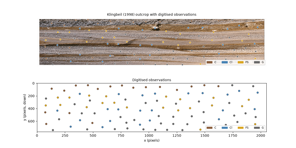
Outcrop photograph and digitised observations

The 100 observation points were digitised directly from the outcrop photograph below. Four lithofacies are visible: gravel and cobble beds (coarse) alternating with fine-sand and clay drapes (fine).

fig, axes = plt.subplots(2, 1, figsize=(12, 6), sharex=True, sharey=True,
                         gridspec_kw={"hspace": 0.35, "height_ratios": [1, 1]})

ax = axes[0]
ax.imshow(img, extent=[0, img_w, img_h, 0], aspect="auto")
for c in cat_labels:
    mask = obs_cats == c
    ax.scatter(obs_coord[mask, 0], obs_coord[mask, 1],
               c=CAT_COLORS[c], s=22, edgecolors="white", linewidths=0.5, zorder=3)
ax.set_title("Klingbeil (1998) outcrop with digitised observations", fontsize=10)
ax.axis("off")
ax.legend(handles=patches, loc="lower right", fontsize=8, ncol=4, framealpha=0.85)

ax = axes[1]
for c in cat_labels:
    mask = obs_cats == c
    ax.scatter(obs_coord[mask, 0], obs_coord[mask, 1],
               c=CAT_COLORS[c], s=30, edgecolors="k", linewidths=0.3, zorder=3)
ax.set_xlim(0, img_w)
ax.set_ylim(img_h, 0)
ax.set_xlabel("x (pixels)")
ax.set_ylabel("y (pixels, down)")
ax.set_title("Digitised observations", fontsize=10)
ax.legend(handles=patches, loc="lower right", fontsize=8, ncol=4, framealpha=0.85)

plt.show()

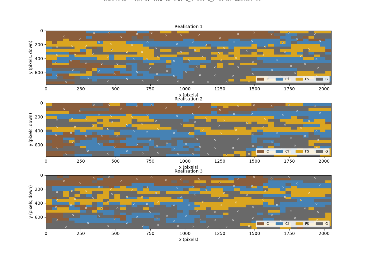
SIS — uniform sill (cross="same")

A single shared sill C₁ = 0.19 ≈ mean(p_k · (1 − p_k)) is used for all K² = 16 variogram pairs. This is the simplest approach and works well in practice because the post_solve normalisation clips and re-weights the K probability estimates to the probability simplex.

ik = IndicatorKriging(
    ncat=ncat, ndim=2, nsim=NSIM,
    neglect_error=True, std_ck=True, seed=SEED,
)
ik.set_categorical_obs(
    coord=obs_coord, categories=obs_cats,
    category_labels=cat_labels, nmax=NMAX,
)
ik.set_indicator_vgm(
    vtype="sph", nugget=NUGGET, sill=SILL,
    a_major=A_MAJOR, a_minor1=A_MINOR, a_minor2=A_MINOR,
    azimuth=AZIMUTH, cross="same",
)
ik.set_grid(coord=grid_coord)
ik.set_sim()
for k in range(1, ncat + 1):
    ik.set_search(ivar=k, anis1=ANIS1, azimuth=AZIMUTH)
ik.solve()

sims_same, _ = ik.get_results()
cat_same     = np.argmax(sims_same, axis=1)   # (n_grid, NSIM) integer index
del ik

fig, axes = plt.subplots(NSIM, 1, figsize=(12, 2.8 * NSIM),
                         gridspec_kw={"hspace": 0.35})
_plot_reals(
    cat_same, axes,
    f"Uniform sill — sph  C₀={NUGGET}  C₁={SILL}"
    f"  a_h={A_MAJOR:.0f}  a_v={A_MINOR:.0f} px  (azimuth={AZIMUTH:.0f}°)",
)
plt.show()

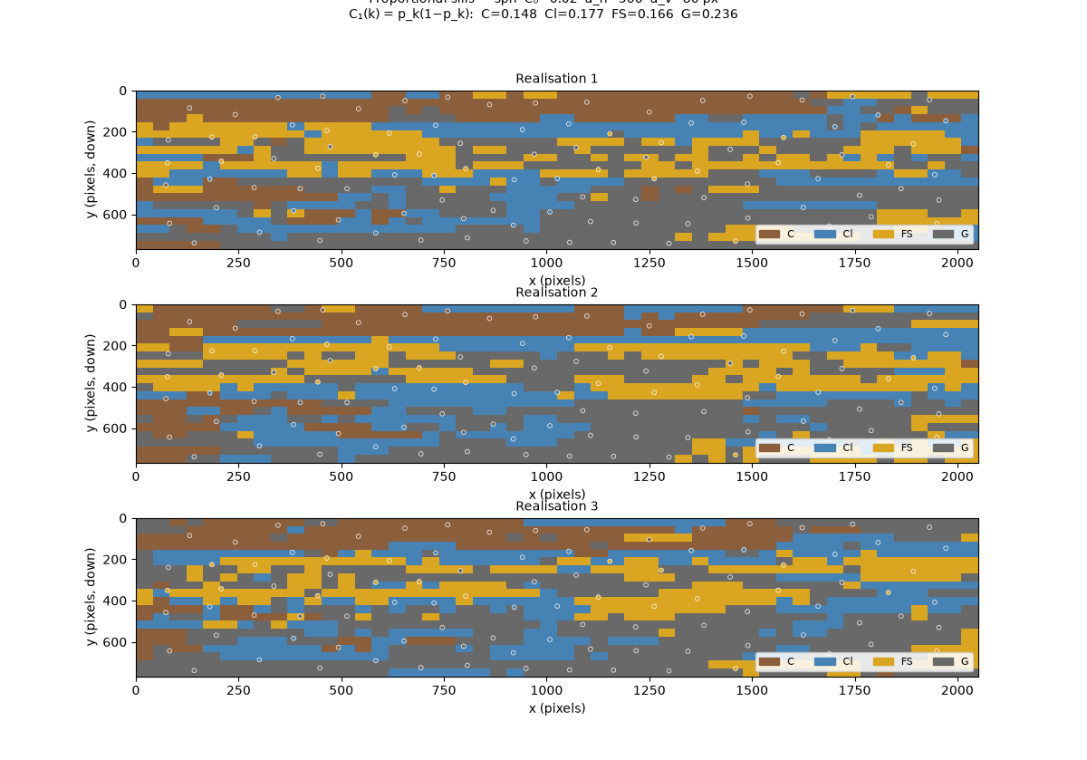
SIS — proportional sills (cross="proportional")

Auto-variogram sills are calibrated to the indicator variance p_k (1 − p_k) for each category. Cross sills are set to √(s_k · s_l) so the coregionalisation matrix is positive-definite for every nested structure (Linear Model of Coregionalisation). The shape (spherical), range, and nugget are shared.

Observed proportions and resulting auto sills:

C  : p = 0.18   C₁ = 0.148
Cl : p = 0.23   C₁ = 0.177
FS : p = 0.21   C₁ = 0.166
G  : p = 0.38   C₁ = 0.236

print("Category proportions and auto sills (p_k · (1 − p_k)):")
for c, p, s in zip(cat_labels, props, auto_sills):
    print(f"  {c:>3s}: p = {p:.3f}   C₁ = {s:.4f}")

ik = IndicatorKriging(
    ncat=ncat, ndim=2, nsim=NSIM,
    neglect_error=True, std_ck=True, seed=SEED,
)
ik.set_categorical_obs(
    coord=obs_coord, categories=obs_cats,
    category_labels=cat_labels, nmax=NMAX,
)
ik.set_indicator_vgm(
    vtype="sph", nugget=NUGGET, sill=SILL,
    a_major=A_MAJOR, a_minor1=A_MINOR, a_minor2=A_MINOR,
    azimuth=AZIMUTH, cross="proportional", proportions=props,
)
ik.set_grid(coord=grid_coord)
ik.set_sim()
for k in range(1, ncat + 1):
    ik.set_search(ivar=k, anis1=ANIS1, azimuth=AZIMUTH)
ik.solve()

sims_prop, _ = ik.get_results()
cat_prop     = np.argmax(sims_prop, axis=1)
del ik

auto_sill_str = "  ".join(f"{c}={s:.3f}" for c, s in zip(cat_labels, auto_sills))
fig, axes = plt.subplots(NSIM, 1, figsize=(12, 2.8 * NSIM),
                         gridspec_kw={"hspace": 0.35})
_plot_reals(
    cat_prop, axes,
    f"Proportional sills — sph  C₀={NUGGET}  a_h={A_MAJOR:.0f}  a_v={A_MINOR:.0f} px"
    f"\nC₁(k) = p_k(1−p_k):  {auto_sill_str}",
)
plt.show()

Category proportions and auto sills (p_k · (1 − p_k)):
    C: p = 0.180   C₁ = 0.1476
   Cl: p = 0.230   C₁ = 0.1771
   FS: p = 0.210   C₁ = 0.1659
    G: p = 0.380   C₁ = 0.2356

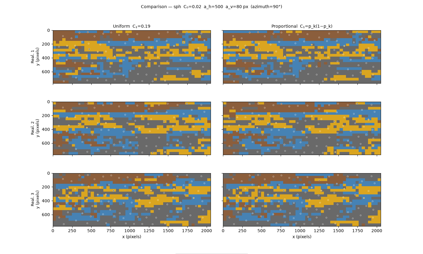
Side-by-side comparison

All three realisations from each cross-variogram strategy are shown together. Left column uses a single shared sill; right column uses category-specific sills calibrated to p_k (1 − p_k). The overall spatial pattern (horizontal continuity, bed thickness) is similar because the variogram shape and range are identical. Differences arise from the changed balance of cross-coupling between indicator variables.

fig, axes = plt.subplots(
    NSIM, 2, figsize=(14, 2.8 * NSIM),
    sharex=True, sharey=True,
    gridspec_kw={"hspace": 0.35, "wspace": 0.08},
)
col_titles = [f"Uniform  C₁={SILL}", "Proportional  C₁=p_k(1−p_k)"]
for col, (cat_idx, col_title) in enumerate(zip([cat_same, cat_prop], col_titles)):
    for row in range(NSIM):
        ax = axes[row, col]
        zz = cat_idx[:, row].reshape(NY, NX)
        ax.imshow(zz, origin="upper", extent=[0, img_w, img_h, 0],
                  cmap=cmap, norm=norm, aspect="auto", interpolation="nearest")
        ax.scatter(obs_coord[:, 0], obs_coord[:, 1],
                   c=[CAT_COLORS[c] for c in obs_cats],
                   s=10, edgecolors="white", linewidths=0.4, zorder=3)
        if col == 0:
            ax.set_ylabel(f"Real. {row + 1}\ny (pixels)", fontsize=9)
        if row == 0:
            ax.set_title(col_title, fontsize=10)
        if row == NSIM - 1:
            ax.set_xlabel("x (pixels)")

fig.legend(handles=patches, loc="lower center", fontsize=8,
           ncol=ncat, bbox_to_anchor=(0.5, -0.03))
fig.suptitle(
    f"Comparison — sph  C₀={NUGGET}  a_h={A_MAJOR:.0f}  a_v={A_MINOR:.0f} px"
    f"  (azimuth={AZIMUTH:.0f}°)",
    fontsize=10,
)
plt.show()