Co-kriging Indicator Simulation with a Continuous Covariate

This example extends Sequential Indicator Simulation of Lithofacies by adding a secondary continuous variable y — a synthetic grain-size proxy — to the indicator co-kriging framework.

The co-kriging MIS uses nvar = ncat + 1 = 5 variables:

• ivar 1–4 — binary indicators for the four lithofacies (same as plain SIS)

• ivar 5 — continuous grain-size index y, sampled at observation locations

y was generated from category-specific Gaussian distributions so that it is correlated with the lithofacies but not perfectly predictable from them:

Code	Lithology	Mean y	σ
G	Gravel	3.0	0.3
C	Cobble	2.5	0.3
FS	Fine Sand	1.0	0.3
Cl	Clay	0.5	0.3

Variogram structure

A 5 × 5 sill matrix couples all variable pairs. For each nested structure j the matrix of partial sills [b_kl^j] must be positive semi-definite (LMC).

• Indicator auto-variograms (k=l, 1–4) — proportional to p_k (1 − p_k)

• Indicator cross-variograms (k≠l, 1–4) — √(s_k · s_l)

• Covariate auto-variogram (5,5) — sample variance of y

• Indicator–covariate cross-variograms (k, 5) — sample covariance cov(I_k, y) (positive for coarse categories, negative for fine categories)

The secondary variable is used to set kriging weights at every grid node but is excluded from the CDF draw and the returned get_results() array.

import numpy as np
import pandas as pd
import matplotlib.pyplot as plt
import matplotlib.patches as mpatches
import matplotlib.colors as mcolors

from krigekit import IndicatorKriging

# ---------------------------------------------------------------------------
# Configuration (shared with s_sis_lithofacies)
# ---------------------------------------------------------------------------

CAT_COL  = "lithologic_code"
X_COL    = "x_pixel"
Y_COL    = "y_pixel0"

NSIM     = 3
NMAX     = 20
SEED     = 42

NX, NY   = 50, 20

NUGGET   = 0.02
SILL     = 0.19
A_MAJOR  = 500.0
A_MINOR  = 80.0
AZIMUTH  = 90.0
ANIS1    = A_MINOR / A_MAJOR

CAT_COLORS = {"C": "#8B5E3C", "Cl": "#4682B4", "FS": "#DAA520", "G": "#696969"}

# Category-specific means for the synthetic grain-size covariate y
GRAIN_MEAN = {"C": 2.5, "Cl": 0.5, "FS": 1.0, "G": 3.0}
GRAIN_SD   = 0.3

# ---------------------------------------------------------------------------
# Load observations, build grid, generate covariate
# ---------------------------------------------------------------------------

df         = pd.read_csv("../test_data/lithofacies.csv")
obs_coord  = df[[X_COL, Y_COL]].values.astype(float)
obs_cats   = df[CAT_COL].values
cat_labels = sorted(df[CAT_COL].unique().tolist())   # ['C', 'Cl', 'FS', 'G']
ncat       = len(cat_labels)
nvar       = ncat + 1                                # 4 indicators + 1 covariate

props      = np.array([df[CAT_COL].eq(c).mean() for c in cat_labels])
auto_sills = props * (1.0 - props)                   # theoretical indicator auto-sills

# Synthetic grain-size covariate y — category mean + Gaussian noise
rng = np.random.default_rng(SEED)
y   = np.array([GRAIN_MEAN[c] for c in obs_cats], dtype=float)
y  += rng.normal(0.0, GRAIN_SD, len(obs_cats))

# Empirical variogram parameters for the covariate
sill_y    = float(np.var(y, ddof=1))
# Sample cross-covariance cov(I_k, y) for k = 1..ncat
indicators = [(obs_cats == c).astype(float) for c in cat_labels]
cross_cov  = np.array([np.cov(ind, y)[0, 1] for ind in indicators])

# Image, grid, shared colourmap
img    = plt.imread("../test_data/lithofacies.png")
img_h, img_w = img.shape[:2]
gx, gy     = np.meshgrid(np.linspace(0, img_w, NX),
                          np.linspace(0, img_h, NY))
grid_coord = np.column_stack([gx.ravel(), gy.ravel()])

cmap    = mcolors.ListedColormap([CAT_COLORS[c] for c in cat_labels])
norm    = mcolors.BoundaryNorm(np.arange(-0.5, ncat, 1.0), cmap.N)
patches = [mpatches.Patch(color=CAT_COLORS[c], label=c) for c in cat_labels]


def _plot_reals(cat_idx, axes, suptitle):
    for i, ax in enumerate(axes):
        zz = cat_idx[:, i].reshape(NY, NX)
        ax.imshow(zz, origin="upper", extent=[0, img_w, img_h, 0],
                  cmap=cmap, norm=norm, aspect="auto", interpolation="nearest")
        ax.scatter(obs_coord[:, 0], obs_coord[:, 1],
                   c=[CAT_COLORS[c] for c in obs_cats],
                   s=12, edgecolors="white", linewidths=0.5, zorder=3)
        ax.set_title(f"Realisation {i + 1}", fontsize=10)
        ax.set_xlabel("x (pixels)")
        ax.set_ylabel("y (pixels, down)")
        ax.legend(handles=patches, loc="lower right", fontsize=8,
                  ncol=4, framealpha=0.85)
    axes[0].get_figure().suptitle(suptitle, fontsize=10, y=1.01)

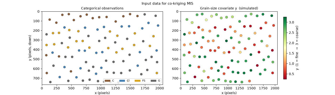
Observations and grain-size covariate y

Left: observations coloured by lithofacies category. Right: the synthetic grain-size index y overlaid on the same locations — warm colours are coarse (gravel / cobble) and cool colours are fine (clay / fine sand). The two panels encode the same 100 points from two perspectives: a discrete categorical label and a continuous proxy.

fig, axes = plt.subplots(1, 2, figsize=(14, 4),
                         gridspec_kw={"wspace": 0.15})

ax = axes[0]
for c in cat_labels:
    mask = obs_cats == c
    ax.scatter(obs_coord[mask, 0], obs_coord[mask, 1],
               c=CAT_COLORS[c], s=45, edgecolors="k", linewidths=0.3, zorder=3)
ax.set_xlim(0, img_w);  ax.set_ylim(img_h, 0)
ax.set_xlabel("x (pixels)");  ax.set_ylabel("y (pixels, down)")
ax.set_title("Categorical observations", fontsize=10)
ax.legend(handles=patches, loc="lower right", fontsize=8, ncol=4, framealpha=0.85)

ax = axes[1]
sc = ax.scatter(obs_coord[:, 0], obs_coord[:, 1],
                c=y, cmap="RdYlGn", vmin=y.min(), vmax=y.max(),
                s=55, edgecolors="k", linewidths=0.3, zorder=3)
ax.set_xlim(0, img_w);  ax.set_ylim(img_h, 0)
ax.set_xlabel("x (pixels)")
ax.set_title("Grain-size covariate y  (simulated)", fontsize=10)
plt.colorbar(sc, ax=ax, label="y  (1 = fine  →  3 = coarse)", shrink=0.85)

fig.suptitle("Input data for co-kriging MIS", fontsize=11)
plt.show()

5 × 5 variogram sill matrix

The sill matrix encodes the spatial coupling between all five variables. Diagonal entries are the auto-sills (variance at large lag). Off-diagonal entries are the cross-sills (cross-covariance at large lag).

Indicator–covariate cross-sills (last column / row) are negative for fine categories because a high grain-size index implies a lower probability of clay or fine sand — exactly the information that co-kriging exploits.

labels_5    = cat_labels + ["y"]
sill_matrix = np.zeros((nvar, nvar))
for k in range(ncat):
    sill_matrix[k, k] = auto_sills[k]
    for l in range(ncat):
        if k != l:
            sill_matrix[k, l] = np.sqrt(auto_sills[k] * auto_sills[l])
sill_matrix[ncat, ncat] = sill_y
for k in range(ncat):
    sill_matrix[k,    ncat] = cross_cov[k]
    sill_matrix[ncat, k   ] = cross_cov[k]

print("5 × 5 variogram sill matrix:")
header = "       " + "  ".join(f"{lb:>7s}" for lb in labels_5)
print(header)
for i, row_label in enumerate(labels_5):
    row = "  ".join(f"{sill_matrix[i, j]:+7.4f}" for j in range(nvar))
    print(f"  {row_label:>3s}  {row}")

fig, ax = plt.subplots(figsize=(5.8, 4.8))
vmax = np.abs(sill_matrix).max()
im   = ax.imshow(sill_matrix, cmap="RdBu_r", vmin=-vmax, vmax=vmax)
ax.set_xticks(range(nvar));  ax.set_xticklabels(labels_5, fontsize=9)
ax.set_yticks(range(nvar));  ax.set_yticklabels(labels_5, fontsize=9)
for i in range(nvar):
    for j in range(nvar):
        ax.text(j, i, f"{sill_matrix[i, j]:+.3f}",
                ha="center", va="center", fontsize=8,
                color="w" if abs(sill_matrix[i, j]) > 0.4 * vmax else "k")
plt.colorbar(im, ax=ax, shrink=0.82)
ax.set_title("Variogram sill matrix  [C₁(ivar, jvar)]", fontsize=10)
plt.show()

5 × 5 variogram sill matrix:
             C       Cl       FS        G        y
    C  +0.1476  +0.1617  +0.1565  +0.1865  +0.1046
   Cl  +0.1617  +0.1771  +0.1714  +0.2043  -0.3138
   FS  +0.1565  +0.1714  +0.1659  +0.1977  -0.1920
    G  +0.1865  +0.2043  +0.1977  +0.2356  +0.4013
    y  +0.1046  -0.3138  -0.1920  +0.4013  +1.1301

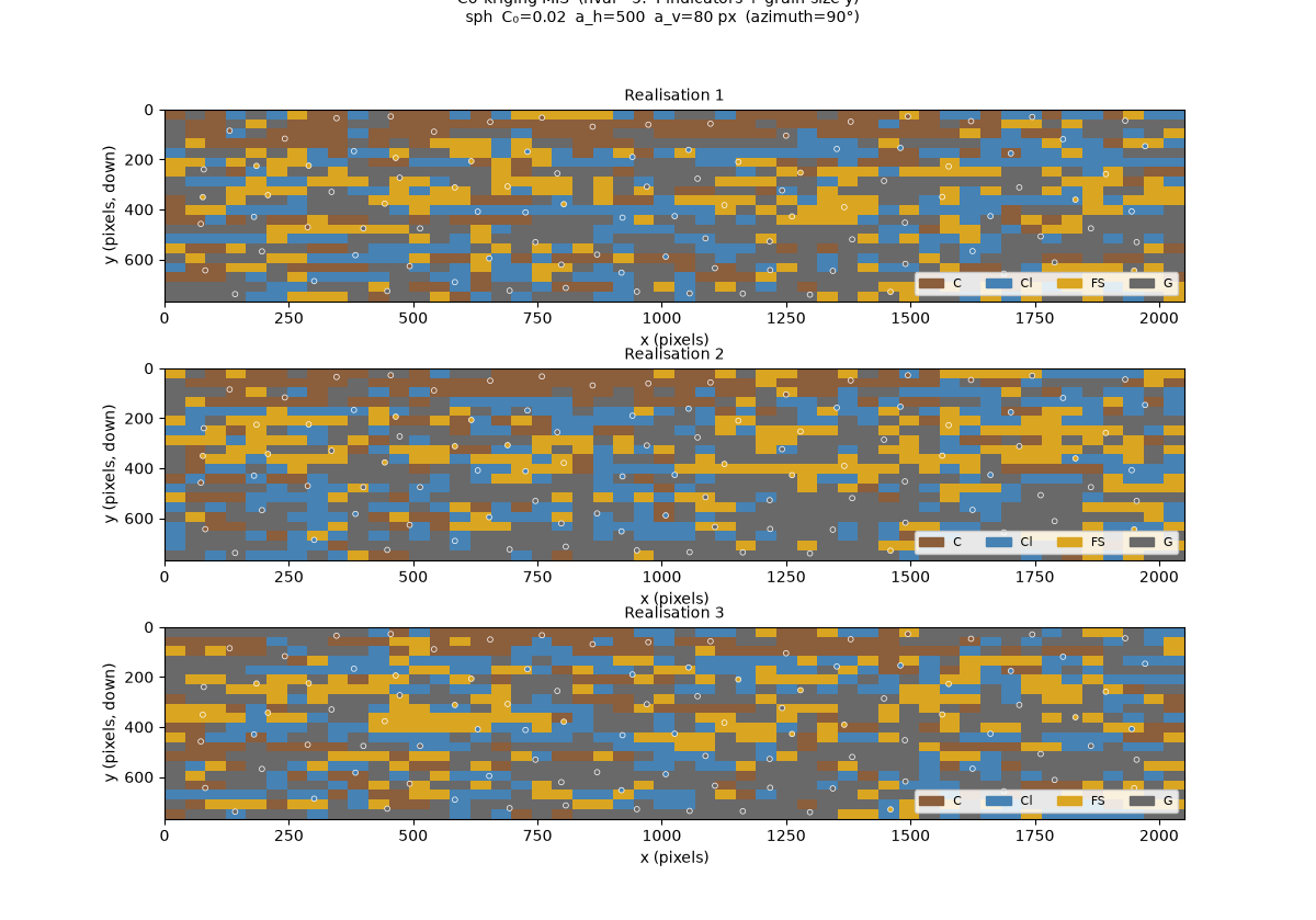
Co-kriging MIS — setup and simulation

IndicatorKriging(ncat=4, nvar=5) allocates a 5 × 5 co-kriging system. The variogram is assembled in three parts:

1. set_indicator_vgm(cross="proportional") — fills the 4 × 4 indicator block.

2. set_vgm(5, 5, ...) — adds the covariate auto-variogram.

3. set_vgm(k, 5, ...) for k = 1–4 — adds the four cross-variograms. Cross-sills for coarse categories are positive; for fine categories negative.

get_results() returns shape (ngrid, nvar, nsim). Only the first ncat slices carry the one-hot indicator draws; the covariate slice is zero everywhere and is dropped with [:, :ncat, :].

ik = IndicatorKriging(
    ncat=ncat, nvar=nvar, ndim=2, nsim=NSIM,
    neglect_error=True, std_ck=True, seed=SEED,
)

# Indicator observations (ivar = 1..ncat)
ik.set_categorical_obs(
    coord=obs_coord, categories=obs_cats,
    category_labels=cat_labels, nmax=NMAX,
)

# Covariate observations (ivar = ncat + 1)
ik.set_obs(ivar=ncat + 1, coord=obs_coord, value=y, nmax=NMAX)

# 4 × 4 indicator block — proportional sills
ik.set_indicator_vgm(
    vtype="sph", nugget=NUGGET, sill=SILL,
    a_major=A_MAJOR, a_minor1=A_MINOR, a_minor2=A_MINOR,
    azimuth=AZIMUTH, cross="proportional", proportions=props,
)

# Covariate auto-variogram (5, 5)
ik.set_vgm(
    ivar=ncat + 1, jvar=ncat + 1,
    vtype="sph", nugget=NUGGET, sill=sill_y,
    a_major=A_MAJOR, a_minor1=A_MINOR, a_minor2=A_MINOR,
    azimuth=AZIMUTH,
)

# Indicator–covariate cross-variograms (k, 5), nugget=0, sill = cov(I_k, y)
# Positive for coarse categories, negative for fine categories.
for k in range(1, ncat + 1):
    ik.set_vgm(
        ivar=k, jvar=ncat + 1,
        vtype="sph", nugget=0.0, sill=float(cross_cov[k - 1]),
        a_major=A_MAJOR, a_minor1=A_MINOR, a_minor2=A_MINOR,
        azimuth=AZIMUTH,
    )

ik.set_grid(coord=grid_coord)
ik.set_sim()

for k in range(1, nvar + 1):
    ik.set_search(ivar=k, anis1=ANIS1, azimuth=AZIMUTH)

ik.solve()

# Shape (ngrid, nvar, NSIM); slice to ncat — covariate slot is zero after draw
sims_coik = ik.get_results()[0][:, :ncat, :]
cat_coik  = np.argmax(sims_coik, axis=1)   # (ngrid, NSIM) integer category index
del ik

fig, axes = plt.subplots(NSIM, 1, figsize=(12, 2.8 * NSIM),
                         gridspec_kw={"hspace": 0.35})
_plot_reals(
    cat_coik, axes,
    f"Co-kriging MIS  (nvar={nvar}: {ncat} indicators + grain-size y)"
    f"\n  sph  C₀={NUGGET}  a_h={A_MAJOR:.0f}  a_v={A_MINOR:.0f} px"
    f"  (azimuth={AZIMUTH:.0f}°)",
)
plt.show()

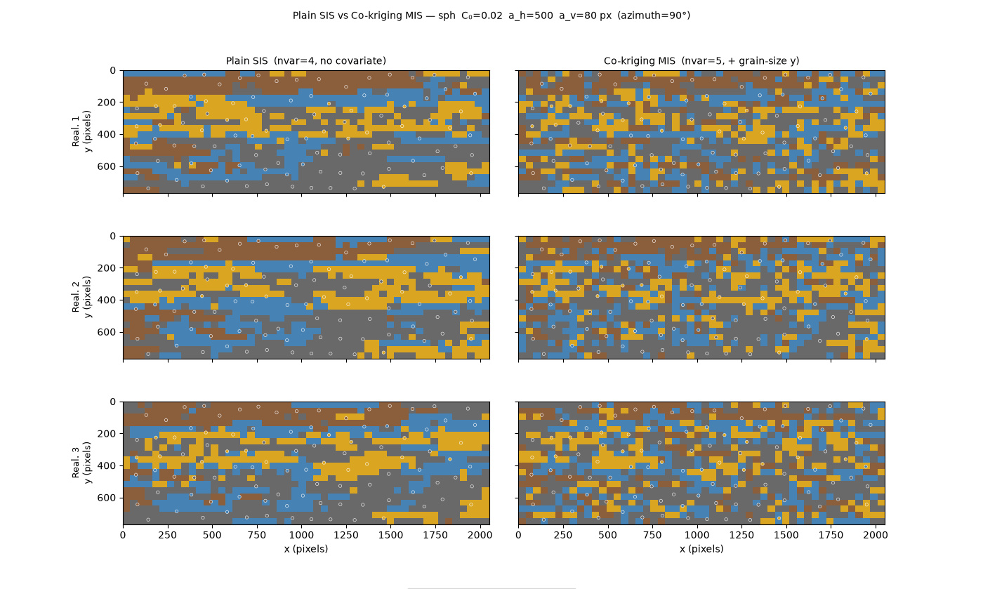
Comparison: plain SIS vs co-kriging MIS

Plain SIS uses only the categorical observations (nvar = ncat = 4) with the same variogram shape and proportional sills. Co-kriging MIS additionally conditions on y at every node, tightening the conditional CDF where the grain-size proxy and the categorical observations agree.

In regions far from observations the covariate has more influence, which can reduce variability between realisations — visible as slightly more coherent bed geometry in the co-kriging column.

ik_plain = IndicatorKriging(
    ncat=ncat, ndim=2, nsim=NSIM,
    neglect_error=True, std_ck=True, seed=SEED,
)
ik_plain.set_categorical_obs(
    coord=obs_coord, categories=obs_cats,
    category_labels=cat_labels, nmax=NMAX,
)
ik_plain.set_indicator_vgm(
    vtype="sph", nugget=NUGGET, sill=SILL,
    a_major=A_MAJOR, a_minor1=A_MINOR, a_minor2=A_MINOR,
    azimuth=AZIMUTH, cross="proportional", proportions=props,
)
ik_plain.set_grid(coord=grid_coord)
ik_plain.set_sim()
for k in range(1, ncat + 1):
    ik_plain.set_search(ivar=k, anis1=ANIS1, azimuth=AZIMUTH)
ik_plain.solve()

sims_plain = ik_plain.get_results()[0]   # (ngrid, ncat, NSIM) when nvar == ncat
cat_plain  = np.argmax(sims_plain, axis=1)
del ik_plain

fig, axes = plt.subplots(
    NSIM, 2, figsize=(14, 2.8 * NSIM),
    sharex=True, sharey=True,
    gridspec_kw={"hspace": 0.35, "wspace": 0.08},
)
col_titles = [
    f"Plain SIS  (nvar={ncat}, no covariate)",
    f"Co-kriging MIS  (nvar={nvar}, + grain-size y)",
]
for col, (cat_idx, col_title) in enumerate(zip([cat_plain, cat_coik], col_titles)):
    for row in range(NSIM):
        ax = axes[row, col]
        zz = cat_idx[:, row].reshape(NY, NX)
        ax.imshow(zz, origin="upper", extent=[0, img_w, img_h, 0],
                  cmap=cmap, norm=norm, aspect="auto", interpolation="nearest")
        ax.scatter(obs_coord[:, 0], obs_coord[:, 1],
                   c=[CAT_COLORS[c] for c in obs_cats],
                   s=10, edgecolors="white", linewidths=0.4, zorder=3)
        if col == 0:
            ax.set_ylabel(f"Real. {row + 1}\ny (pixels)", fontsize=9)
        if row == 0:
            ax.set_title(col_title, fontsize=10)
        if row == NSIM - 1:
            ax.set_xlabel("x (pixels)")

fig.legend(handles=patches, loc="lower center", fontsize=8,
           ncol=ncat, bbox_to_anchor=(0.5, -0.03))
fig.suptitle(
    f"Plain SIS vs Co-kriging MIS — sph  C₀={NUGGET}"
    f"  a_h={A_MAJOR:.0f}  a_v={A_MINOR:.0f} px  (azimuth={AZIMUTH:.0f}°)",
    fontsize=10,
)
plt.show()