Ordinary kriging example

This example shows how to run ordinary kriging and plot the interpolated field.

from krigekit import Kriging
import pandas as pd
import matplotlib.pyplot as plt

data = pd.read_csv("../test_data/pc2d.csv")
grid = pd.read_csv("../test_data/grid2d.csv")

# default is 2D univariate ordinary Kriging
k = Kriging()
k.set_obs(ivar=1, coord=data[["x", "y"]], value=data["pc"], nmax=30)
k.set_grid(coord=grid[["x", "y"]])
k.set_vgm(ivar=1, jvar=1, vtype="sph", sill=0.12, a_major=5000.0)
k.set_search()
k.solve()
df = k.get_result_df()

print(df)

             x          y  estimate  variance
0     573349.0  4400382.0  0.946436  0.051236
1     573554.0  4400525.0  0.903184  0.055179
2     573759.0  4400669.0  0.852546  0.056888
3     573964.0  4400812.0  0.794709  0.056655
4     574169.0  4400956.0  0.729639  0.054859
...        ...        ...       ...       ...
4795  595941.0  4392091.0  0.711334  0.048720
4796  596146.0  4392234.0  0.712876  0.039330
4797  596351.0  4392377.0  0.714335  0.029492
4798  596555.0  4392521.0  0.711500  0.022719
4799  596760.0  4392664.0  0.698329  0.024836

[4800 rows x 4 columns]

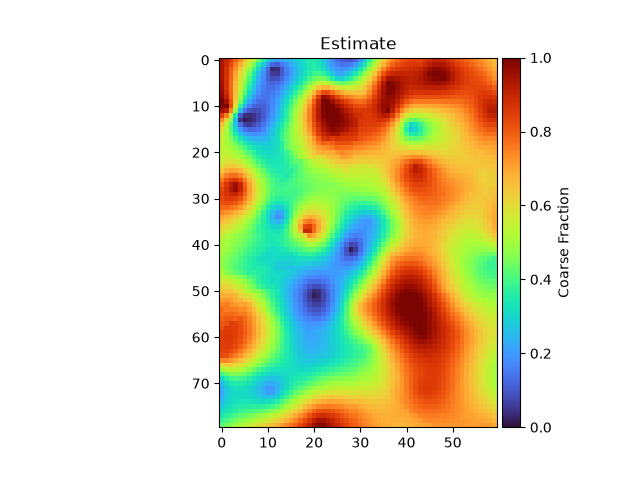
Plot the interpolated values

plt.imshow(df["estimate"].values.reshape([80, 60]), cmap="turbo", vmin=0, vmax=1)
plt.title("Estimate")
plt.colorbar(label="Coarse Fraction", pad=0.01)
plt.show()

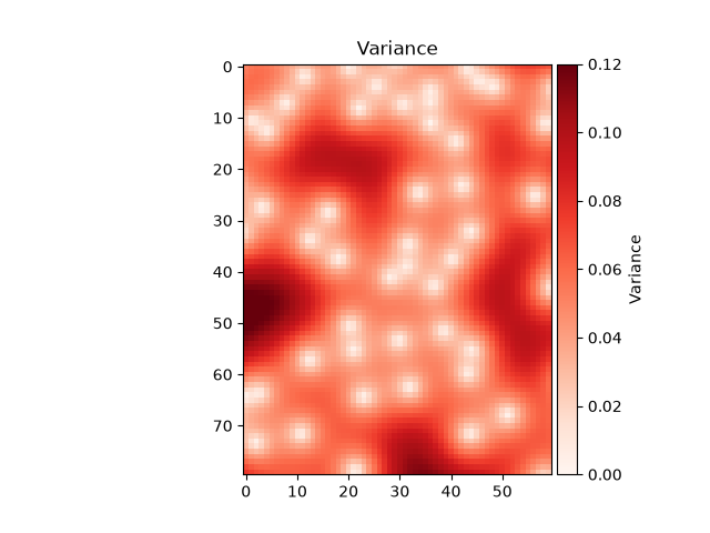
Plot the Kriging error

plt.imshow(df["variance"].values.reshape([80, 60]), cmap="Reds", vmin=0, vmax=0.12)
plt.title("Variance")
plt.colorbar(label="Variance", pad=0.01)
plt.show()