Co-kriging the Walker Lake dataset

Co-kriging estimates a sparsely sampled primary variable by borrowing strength from a densely sampled secondary variable through a cross-variogram.

Dataset — Walker Lake (Isaaks & Srivastava, 1989, An Introduction to Applied Geostatistics, ch. 17):

• U — primary variable, 275 observations (sparse).

• V — secondary variable, 470 observations (abundant).

Both variables occupy a 260 × 300 unit domain. In regions where U is unsampled, V measurements constrain the estimate through the cross-variogram.

Linear Model of Coregionalisation (LMC) — two nested spherical structures with geometric anisotropy (azimuth 14°, major range / minor range = 2 : 1):

γ_U (h) =  22 000  +  40 000·Sph₁(h)  +  45 000·Sph₂(h)
γ_V (h) = 440 000  +  70 000·Sph₁(h)  +  95 000·Sph₂(h)
γ_UV(h) =  47 000  +  50 000·Sph₁(h)  +  40 000·Sph₂(h)

LMC validity (C₁₂² ≤ C₁₁ · C₂₂ per structure):

• Nugget: 47 000² = 2.21×10⁹ ≤ 22 000 × 440 000 = 9.68×10⁹ ✓

• Structure 1: 50 000² = 2.50×10⁹ ≤ 40 000 × 70 000 = 2.80×10⁹ ✓

• Structure 2: 40 000² = 1.60×10⁹ ≤ 45 000 × 95 000 = 4.28×10⁹ ✓

import numpy as np
import pandas as pd
import matplotlib.pyplot as plt
from krigekit import Kriging

# ---------------------------------------------------------------------------
# Load data (Isaaks & Srivastava 1989 case study setup)
# ---------------------------------------------------------------------------
df      = pd.read_csv("../test_data/walker.csv")
mask_u  = df["U"] != -999

coord_v = df[["X", "Y"]].values.astype(float)              # V: all 470 obs
val_v   = df["V"].values.astype(float)
coord_u = df.loc[mask_u, ["X", "Y"]].values.astype(float)  # U: 275 obs
val_u   = df.loc[mask_u, "U"].values.astype(float)

# 25 × 30 estimation grid over [10, 250] × [10, 290]
NX, NY     = 25, 30
gx, gy     = np.meshgrid(np.linspace(10, 250, NX), np.linspace(10, 290, NY))
grid_coord = np.column_stack([gx.ravel(), gy.ravel()])

# ---------------------------------------------------------------------------
# Variogram parameters (Isaaks & Srivastava 1989, Eq. 17.11–17.14)
# ---------------------------------------------------------------------------
_AZ = 14.0   # azimuth (°): major axis 14° clockwise from North

_VGM_UU = [
    dict(vtype="sph", nugget=22000, sill=40000,
         a_major=40.0,  a_minor1=20.0, a_minor2=40.0,  azimuth=_AZ),
    dict(vtype="sph", nugget=0,     sill=45000,
         a_major=150.0, a_minor1=100.0, a_minor2=150.0, azimuth=_AZ),
]
_VGM_VV = [
    dict(vtype="sph", nugget=440000, sill=70000,
         a_major=40.0,  a_minor1=20.0, a_minor2=40.0,  azimuth=_AZ),
    dict(vtype="sph", nugget=0,      sill=95000,
         a_major=150.0, a_minor1=100.0, a_minor2=150.0, azimuth=_AZ),
]
_VGM_UV = [
    dict(vtype="sph", nugget=47000, sill=50000,
         a_major=40.0,  a_minor1=20.0, a_minor2=40.0,  azimuth=_AZ),
    dict(vtype="sph", nugget=0,     sill=40000,
         a_major=150.0, a_minor1=100.0, a_minor2=150.0, azimuth=_AZ),
]

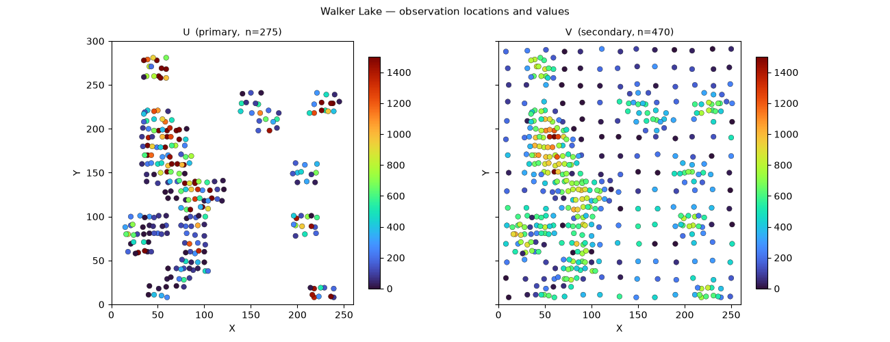
Observations

U (primary, sparse) and V (secondary, abundant) are shown side-by-side. Where U is absent, V provides indirect information through the cross-variogram.

fig, axes = plt.subplots(1, 2, figsize=(13, 5),
                         sharex=True, sharey=True,
                         gridspec_kw={"wspace": 0.28})

for ax, coord, val, label in zip(
        axes,
        [coord_u,                 coord_v],
        [val_u,                   val_v],
        [f"U  (primary,  n={len(val_u)})", f"V  (secondary, n={len(val_v)})"]):
    sc = ax.scatter(coord[:, 0], coord[:, 1], c=val,
                    cmap="turbo", vmin=0, vmax=1500,
                    s=30, edgecolors="k", linewidths=0.25, zorder=3)
    plt.colorbar(sc, ax=ax, shrink=0.88)
    ax.set_xlim(0, 260);  ax.set_ylim(0, 300)
    ax.set_xlabel("X");   ax.set_ylabel("Y")
    ax.set_title(label, fontsize=10)

fig.suptitle("Walker Lake — observation locations and values", fontsize=11)
plt.show()

Ordinary kriging of U

Kriging U alone, without using V. High variance wherever U observations are absent.

k_ok = Kriging(ndim=2, nvar=1)
k_ok.set_obs(ivar=1, coord=coord_u, value=val_u, nmax=20)
for spec in _VGM_UU:
    k_ok.set_vgm(ivar=1, jvar=1, **spec)
k_ok.set_grid(coord=grid_coord)
k_ok.set_search(ivar=1)
k_ok.solve()
est_ok, var_ok = k_ok.get_results()
del k_ok

print(f"OK      — mean variance = {var_ok.mean():,.0f}")

OK      — mean variance = 74,595

Co-kriging U with V

V (ivar=2) supplies information at U-unsampled locations through the cross-variogram. set_vgm(1, 2, ...) sets the cross-variogram between U and V; the LMC requires symmetric specification (set for ivar ≤ jvar).

k_cok = Kriging(ndim=2, nvar=2)
k_cok.set_obs(ivar=1, coord=coord_u, value=val_u, nmax=20)  # U = primary
k_cok.set_obs(ivar=2, coord=coord_v, value=val_v, nmax=20)  # V = secondary
for spec in _VGM_UU:
    k_cok.set_vgm(ivar=1, jvar=1, **spec)
for spec in _VGM_VV:
    k_cok.set_vgm(ivar=2, jvar=2, **spec)
for spec in _VGM_UV:
    k_cok.set_vgm(ivar=1, jvar=2, **spec)
k_cok.set_grid(coord=grid_coord)
k_cok.set_search(ivar=1)
k_cok.set_search(ivar=2)
k_cok.solve()

# get_results() returns (ngrid, nvar) estimate and (ngrid, nvar, nvar) covariance
all_est, all_var = k_cok.get_results()
est_cok = all_est[:, 0]      # U estimate (ivar=1)
var_cok = all_var[:, 0, 0]   # U kriging variance
del k_cok

var_reduction = 100.0 * (1.0 - var_cok.mean() / var_ok.mean())
print(f"Co-kriging — mean variance = {var_cok.mean():,.0f}  "
      f"(reduction: {var_reduction:.1f}%)")

Co-kriging — mean variance = 67,934  (reduction: 8.9%)

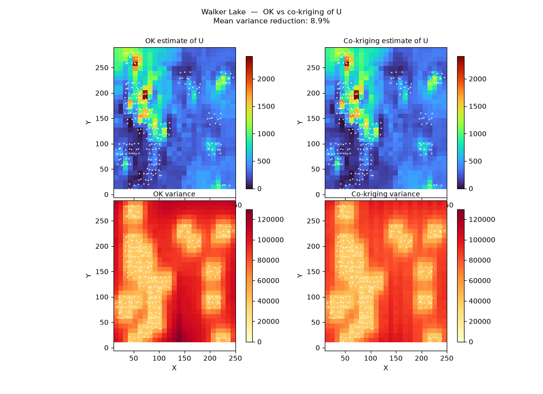
Comparison: OK vs co-kriging

The upper row shows estimates; the lower row shows kriging variances. Co-kriging (right column) borrows V’s dense coverage to reduce the variance in regions where U is unobserved.

vmax_est = max(est_ok.max(), est_cok.max())
vmax_var = var_ok.max()

fig, axes = plt.subplots(2, 2, figsize=(11, 8),
                         gridspec_kw={"hspace": 0.02, "wspace": 0.01})

for ax, data, title, cmap, vmax in [
    (axes[0, 0], est_ok,  "OK estimate of U",        "turbo",  vmax_est),
    (axes[0, 1], est_cok, "Co-kriging estimate of U", "turbo",  vmax_est),
    (axes[1, 0], var_ok,  "OK variance",              "YlOrRd", vmax_var),
    (axes[1, 1], var_cok, "Co-kriging variance",      "YlOrRd", vmax_var),
]:
    im = ax.imshow(data.reshape(NY, NX), cmap=cmap, vmin=0, vmax=vmax,
                   origin="lower", extent=[10, 250, 10, 290])
    plt.colorbar(im, ax=ax, shrink=0.88)
    ax.scatter(coord_u[:, 0], coord_u[:, 1],
               c="white", s=5, lw=0, zorder=3, alpha=0.7)
    ax.set_xlabel("X");  ax.set_ylabel("Y")
    ax.set_aspect("equal")
    ax.set_title(title, fontsize=10)

fig.suptitle(
    f"Walker Lake  —  OK vs co-kriging of U\n"
    f"Mean variance reduction: {var_reduction:.1f}%",
    fontsize=11,
)
plt.show()