Leave-one-out cross-validation

Cross-validation checks whether a variogram model is consistent with the data by predicting each observation from its neighbours, leaving it out of the kriging system.

Two diagnostics are used:

• RMSE (root-mean-squared error) — how close estimates are to the observed values.

• MSSE (mean standardised squared error) = mean((obs − est)² / var_cv). A well-calibrated model gives MSSE ≈ 1. MSSE > 1 means the variogram underestimates prediction uncertainty (too optimistic); MSSE < 1 means it overestimates it.

Workflow — set cross_validation=True in the constructor and call set_grid_cv() instead of set_grid(). krigekit then returns one estimate and one variance per observation.

Dataset — pc2d.csv: 62 percent-coarse observations on a 2-D spatial domain. Variogram: spherical, nugget = 0, sill = 0.12, range = 5 000 m (isotropic).

import numpy as np
import pandas as pd
import matplotlib.pyplot as plt
from krigekit import Kriging

data = pd.read_csv("../test_data/pc2d.csv")
grid = pd.read_csv("../test_data/grid2d.csv")

obs_coord = data[["x", "y"]].values
obs_value = data["pc"].values

VGM = dict(vtype="sph", nugget=0.0, sill=0.12, a_major=5000.0)

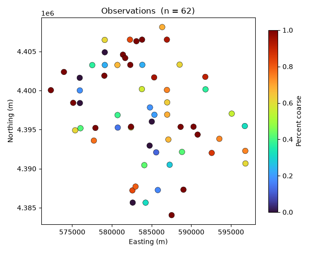
Observations

62 percent-coarse measurements at irregular locations over a ~50 km domain.

fig, ax = plt.subplots(figsize=(6.5, 5.2))
sc = ax.scatter(obs_coord[:, 0], obs_coord[:, 1],
                c=obs_value, cmap="turbo", vmin=0, vmax=1,
                s=70, edgecolors="k", linewidths=0.4, zorder=3)
plt.colorbar(sc, ax=ax, label="Percent coarse", shrink=0.88)
ax.set_xlabel("Easting (m)")
ax.set_ylabel("Northing (m)")
ax.set_title(f"Observations  (n = {len(obs_value)})")
plt.tight_layout()
plt.show()

LOO cross-validation

Setting nmax to the full dataset size (or leaving it unlimited) uses all observations as potential neighbours, matching the reference LOO-CV column in pc2d.csv.

k = Kriging(cross_validation=True)
k.set_obs(ivar=1, coord=obs_coord, value=obs_value)   # no nmax limit
k.set_vgm(ivar=1, jvar=1, **VGM)
k.set_grid_cv()
k.set_search()
k.solve()
est_cv, var_cv = k.get_results()
del k

residuals = obs_value - est_cv
rmse      = np.sqrt(np.mean(residuals ** 2))
r         = np.corrcoef(obs_value, est_cv)[0, 1]
std_resid = residuals / np.sqrt(var_cv)
msse      = np.mean(std_resid ** 2)

print(f"LOO-CV  RMSE = {rmse:.4f}   r = {r:.4f}   MSSE = {msse:.2f}")

fig, axes = plt.subplots(1, 2, figsize=(12, 4.8),
                         gridspec_kw={"wspace": 0.35})

ax = axes[0]
ax.scatter(obs_value, est_cv, s=50, edgecolors="k",
           linewidths=0.35, alpha=0.85)
ax.plot([0, 1], [0, 1], "r--", lw=1.2, label="1:1 line")
ax.set_xlim(0, 1);  ax.set_ylim(0, 1)
ax.set_xlabel("Observed (percent coarse)")
ax.set_ylabel("LOO-CV estimate")
ax.set_title(f"Observed vs LOO-CV\n r = {r:.3f},  RMSE = {rmse:.4f}")
ax.legend(fontsize=9)

ax = axes[1]
ax.hist(std_resid, bins=10, edgecolor="k", linewidth=0.5, alpha=0.85)
ax.axvline(0, color="r", linestyle="--", linewidth=1.2)
ax.set_xlabel("Standardised residual  z = (obs − est) / √var")
ax.set_ylabel("Count")
ax.set_title(f"Standardised residuals\nMSSE = {msse:.2f}  (well-calibrated ≈ 1)")
plt.tight_layout()
plt.show()

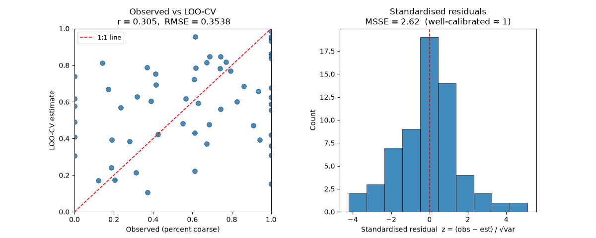
LOO-CV  RMSE = 0.3538   r = 0.3055   MSSE = 2.62
/home/docs/checkouts/readthedocs.org/user_builds/pykriging/checkouts/stable/examples/s_cross_validation.py:100: UserWarning: This figure includes Axes that are not compatible with tight_layout, so results might be incorrect.
  plt.tight_layout()