Kriging with External Drift — groundwater levels

Kriging with External Drift (KED), also called Universal Kriging with a known trend, incorporates a secondary variable available at all prediction locations to model a non-stationary mean.

In this example the drift function is the land-surface elevation (DEM), which correlates strongly with groundwater levels (r ≈ 0.99). Plain ordinary kriging (OK) assumes a stationary mean and ignores this structure; KED explicitly conditions each estimate on the local elevation, producing maps that track the topographic gradient far more faithfully.

Workflow

1. Call Kriging(ndrift=1) to declare one external drift function.

2. Supply drift values at observation locations with set_obs_drift().

3. Supply drift values at grid nodes with set_grid_drift().

4. The variogram is fitted to the residuals after removing the linear DEM trend — these represent the spatially correlated component unexplained by the drift.

Dataset — obs_gwlevel.csv: 334 groundwater-level observations from wells in 2015. Column dem35 is the land-surface elevation at each well. The DEM is interpolated to grid nodes by nearest-neighbour.

import numpy as np
import pandas as pd
import matplotlib.pyplot as plt
from scipy.interpolate import NearestNDInterpolator
from krigekit import Kriging

# ---------------------------------------------------------------------------
# Load 2015 observations
# ---------------------------------------------------------------------------
df   = pd.read_csv("../test_data/obs_gwlevel.csv")
df15 = df[df["Year"] == 2015].dropna(subset=["Observed", "dem35"])

obs_coord = df15[["x", "y"]].values.astype(float)
obs_wl    = df15["Observed"].values.astype(float)   # groundwater level (m)
obs_dem   = df15["dem35"].values.astype(float)       # land-surface elevation (m)

r_wl_dem = np.corrcoef(obs_wl, obs_dem)[0, 1]
print(f"N = {len(obs_wl)} wells  |  r(water level, DEM) = {r_wl_dem:.3f}")

# Variogram of residuals after removing the linear DEM trend
A        = np.column_stack([obs_dem, np.ones(len(obs_dem))])
coeff, _, _, _ = np.linalg.lstsq(A, obs_wl, rcond=None)
resid    = obs_wl - A @ coeff
sill_res = float(np.var(resid, ddof=1))
sill_tot = float(np.var(obs_wl, ddof=1))
print(f"Total variance = {sill_tot:.1f} m²  →  "
      f"residual variance (after DEM detrend) = {sill_res:.1f} m²  "
      f"(R² = {1 - sill_res / sill_tot:.3f})")

# ---------------------------------------------------------------------------
# Estimation grid — 40 × 30 = 1 200 nodes
# ---------------------------------------------------------------------------
NX, NY = 40, 30
x_rng  = obs_coord[:, 0].min(), obs_coord[:, 0].max()
y_rng  = obs_coord[:, 1].min(), obs_coord[:, 1].max()
gx, gy = np.meshgrid(np.linspace(*x_rng, NX),
                     np.linspace(*y_rng, NY))
grid_coord = np.column_stack([gx.ravel(), gy.ravel()])

# DEM at grid nodes — nearest-neighbour interpolation from wells
dem_nn   = NearestNDInterpolator(obs_coord, obs_dem)
grid_dem = dem_nn(grid_coord)

# OK uses the total data sill; KED uses the residual sill (unexplained by drift).
# Using the same sill for both would make OK artificially optimistic — the full
# spatial variability of water levels is much larger than the post-drift residual.
VGM_OK  = dict(vtype="sph", nugget=0.0, sill=sill_tot, a_major=200_000.0)
VGM_KED = dict(vtype="sph", nugget=0.0, sill=max(sill_res, 50.0), a_major=200_000.0)
NMAX = 25

N = 334 wells  |  r(water level, DEM) = 0.991
Total variance = 86475.8 m²  →  residual variance (after DEM detrend) = 1581.0 m²  (R² = 0.982)

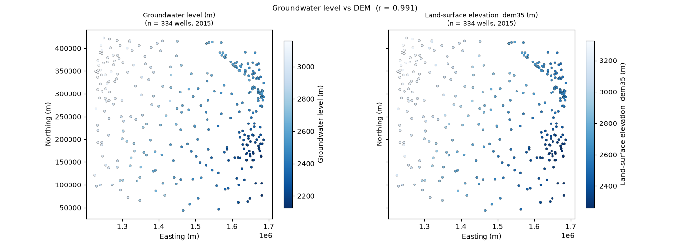
Observations

334 wells from 2015 coloured by groundwater level (left) and land-surface elevation (right). The near-perfect correlation means elevation is an effective proxy for the groundwater trend.

fig, axes = plt.subplots(1, 2, figsize=(14, 5),
                         sharex=True, sharey=True,
                         gridspec_kw={"wspace": 0.30})

for ax, values, label in zip(axes,
        [obs_wl,  obs_dem],
        ["Groundwater level (m)",    "Land-surface elevation  dem35 (m)"]):
    vmin_v, vmax_v = values.min(), values.max()
    sc = ax.scatter(obs_coord[:, 0], obs_coord[:, 1],
                    c=values, cmap="Blues_r", vmin=vmin_v, vmax=vmax_v,
                    s=12, edgecolors="k", linewidths=0.2, zorder=3)
    plt.colorbar(sc, ax=ax, label=label, shrink=0.88)
    ax.set_xlabel("Easting (m)")
    ax.set_ylabel("Northing (m)")
    ax.set_title(f"{label}\n(n = {len(obs_wl)} wells, 2015)", fontsize=9)

fig.suptitle(f"Groundwater level vs DEM  (r = {r_wl_dem:.3f})", fontsize=11)
plt.show()

Ordinary kriging

OK assumes a constant (but unknown) mean and smooths the water levels without accounting for the elevation gradient.

k_ok = Kriging()
k_ok.set_obs(ivar=1, coord=obs_coord, value=obs_wl, nmax=NMAX)
k_ok.set_vgm(ivar=1, jvar=1, **VGM_OK)
k_ok.set_grid(coord=grid_coord)
k_ok.set_search()
k_ok.solve()
est_ok, var_ok = k_ok.get_results()
del k_ok

Kriging with External Drift

ndrift=1 adds the DEM as an external drift function. set_obs_drift supplies DEM values at well locations; set_grid_drift supplies them at grid nodes. The variogram (VGM_KED) is fitted to the residuals after removing the linear DEM trend — a much smaller sill than the total data variance.

k_ked = Kriging(ndrift=1)
k_ked.set_obs(ivar=1, coord=obs_coord, value=obs_wl, nmax=NMAX)
k_ked.set_obs_drift(ivar=1, drift=obs_dem.reshape(-1, 1))  # shape (nobs, 1)
k_ked.set_vgm(ivar=1, jvar=1, **VGM_KED)
k_ked.set_grid(coord=grid_coord)
k_ked.set_grid_drift(drift=grid_dem.reshape(-1, 1))        # shape (ngrid, 1)
k_ked.set_search()
k_ked.solve()
est_ked, var_ked = k_ked.get_results()
del k_ked

print(f"OK  mean variance = {var_ok.mean():,.0f} m²  (sill = {sill_tot:.0f} m²)")
print(f"KED mean variance = {var_ked.mean():,.0f} m²  (sill = {sill_res:.0f} m²)")

OK  mean variance = 10,564 m²  (sill = 86476 m²)
KED mean variance = 204 m²  (sill = 1581 m²)

OK vs KED — estimates and variances

Upper row: estimates. OK (left) produces a gentle smoothed surface; KED (right) tracks the topographic gradient because elevation is baked into the kriging equations at every grid node. Lower row: variances — the KED variogram uses the residual sill (≈ 2 % of total variance), so its variance is much smaller than OK’s, which accounts for the full unexplained spatial variability.

ext = [x_rng[0], x_rng[1], y_rng[0], y_rng[1]]

fig, axes = plt.subplots(2, 2, figsize=(14, 9),
                         gridspec_kw={"hspace": 0.40, "wspace": 0.30})

# Estimate panels share colorbar limits; variance panels use independent scales
# (OK sill >> KED sill, so a shared scale would hide all KED structure).
est_lo = min(est_ok.min(), est_ked.min())
est_hi = max(est_ok.max(), est_ked.max())

for ax, data, title, cmap, v0, v1 in [
    (axes[0, 0], est_ok,  "OK estimate (m)",                        "Blues_r", est_lo,       est_hi),
    (axes[0, 1], est_ked, "KED estimate (m)",                       "Blues_r", est_lo,       est_hi),
    (axes[1, 0], var_ok,  f"OK variance (m²)  [sill={sill_tot:.0f}]",  "YlOrRd", 0, var_ok.max()),
    (axes[1, 1], var_ked, f"KED variance (m²) [sill={sill_res:.0f}]",  "YlOrRd", 0, var_ked.max()),
]:
    im = ax.imshow(data.reshape(NY, NX), cmap=cmap, vmin=v0, vmax=v1,
                   origin="lower", extent=ext, aspect="auto")
    plt.colorbar(im, ax=ax, shrink=0.88)
    ax.scatter(obs_coord[:, 0], obs_coord[:, 1],
               c="k", s=3, lw=0, zorder=3, alpha=0.4)
    ax.set_title(title, fontsize=10)
    ax.set_xlabel("Easting (m)")
    ax.set_ylabel("Northing (m)")

fig.suptitle(
    "Ordinary Kriging vs Kriging with External Drift\n"
    "2015 groundwater levels — elevation as drift function",
    fontsize=11,
)
plt.show()